Before I will post Part 2 of our Havelock travel time modelling exercise, I would like to address the following feedback from Paul:
The starting point is the assumption that VIA's Siemens equipment will be the benchmark equipment for this run.
My first key assumption is that its performance envelope will prove to be similar to the "InterCity" equipment cited in
@Urban Sky's thesis. The important point is the acceleration/deceleration parameter - 0.37m/sec^2. I am using that statistic for all my calculations of acceleration and deceleration on the line. That number may not be reality, but it's a sensible figure to use, and it aligns to
@Urban Sky's work.
Second, I am assuming that deceleration and acceleration rates should be treated as the same.... again, that may not be the case, but it's a conservative assumption for modelling.
We need to be clear as to why we make these calculations: my starting point is that
@reaperexpress claimed that is physically impossible to achieve a better travel time than 3:40 (i.e. 25 minutes slower than the HFR target time promise) and that even that travel time could not be achieved under the constraints inherent to real-world operations. Therefore, I'm not trying to prove that 3:15 can be achieved with little or no alterations to the existing alignment, but to show that claims that such a travel time would be achievable are reasonably credible. This means that I'm making relatively aggressive (but not implausible) assumptions and I will hand over the spreadsheet to you two (and anyone else interested) to play with the various parameters until you believe that the results are reasonably dependable to assume that such a travel time might very well be achievable. It's fine if you insist in changing the deceleration value to something smaller as soon as you get your hand onto it, but at this point, I'm refusing to use performance variables which are only half of the lowest values I identified (for the purposes of my Thesis) in the table I posted in response to nfitz
earlier today.
Finally, I am assuming that the superelevation that VIA can achieve on curves is, as noted in above posts, 8 inches total - three unbalanced and five balanced. While there is freight traffic west of Havelock, let's assume its volume is not so great to force lower superelevation. Using
this FRA chart, the good news is, I can assume that a 3 degree curve can be negotiated at 60 mph. (I am doing all my work in miles rather than kilometers, so as to align to railway mileposts....it just keeps the source data readable). Since 3 degree curves are the most problemmatic limiting curve, 60 mph becomes the "worst case" for speed, other than in a few sections where either curvature is extraordinary or speed may be restricted for other reasons eg in urban areas.
As I showed with the example of Brightline, 8 (i.e. 5+3) inches of superelevation seems to be a realistic assumption...
That's not all bad news, considering that highway speeds are comparable, and the 60 mph prevailing speed is a lot better than I had feared (I had figured most curves would be in the 50 mph range). So end to end times may prove to be fairly competitive to bus or car. (EDIT: This is most true east of Tweed; west of there there are certainly some credible 110 mph capable segments)
I'm glad we agree on this already...!
The practical problem this creates is that, in the absence of a sophisticated autopilot, a train run by human hand will have difficulty handling all the changes in speed to extract the optimum speed-up/slow-down cycles required. Further, the number of full throttle-followed-by-heavy-braking cycles are not condusive to equipment SOGR or fuel efficiency. The likely solution will be to impose "zone" speeds which limit speed over the short tangent stretches to something close to or equal to the slow points of the curves.
Indeed, these frequent changes in speed limits would be impractical with VIA's current fleet, but with a semi-automated train operation system (see table below) like PTC, it should be possible to have the train adjust the speed to stay within any relevant speed limits at any given time (i.e. forcing the train to break before a more restrictive speed limit takes effect).
Quoted in:
my Master Thesis (p.56)
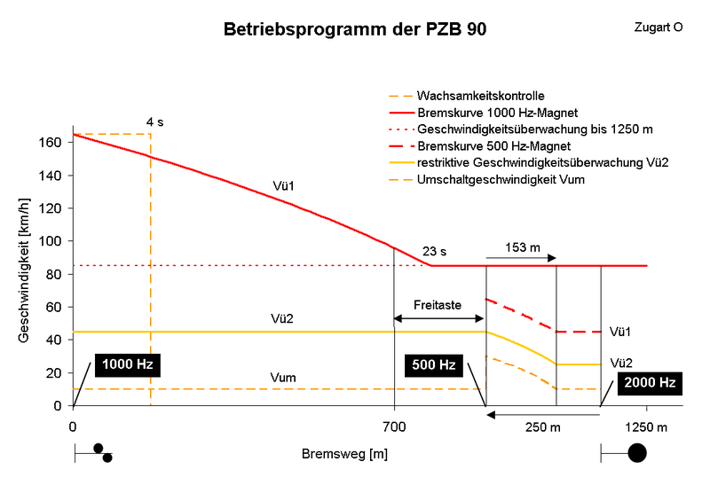
In Germany, all conventional lines are equipped with a GOA 1 system called "
PZB", where magnets resonating at variable frequencies (500, 1000 or 2000 Hz) communicate basic signal configurations:
Source:
Wikipedia
Consequently, a 1000 Hz magnet (located at a pre-signal) is active whenever the following signal is in a restrictive ("slow" or "stop") state and the 500 Hz (located in front of a full signal) and 2000 Hz (located immediately at said full signal) are active when the signal shows a "stop". If you ever want to see that system in action, pay a visit to Ottawa, sit near the cab on the Trillium line and listen to the beeps every time the train runs over a yellow magnet (attached to the right of the tracks) - you will also notice that the system has never been made for systems where you constantly encounter active magnets (given that every signal either protects a passing section or a terminus station).
However, for all trains exceeding speeds of 160 km/h (100 mph), there is a different system (
LZB), which continuously communicates with the train and allows for an autopilot, where the system accelerates or decelerates automatically to the maximum safe speed (given current and future speed limits) or the maximum speed which has been set by the driver (whichever is lower). PZB was conceived in the 1930s and LZB in the 1960s, so neither system is revolutionary and they both get currently superseded (just like all other national legacy systems in Europe) by the universal
ETCS standard.
Please, critique the above to shreds..... I'm still working on the granular picture, better now before I have to rework stuff.
- Paul
This is already really good work, but no worries, I will share my spreadsheet as soon as I have presented it here, so no need to duplicate the efforts...!